Dimensional analysis and blasts from the past

It’s a summer of cleaning out a lot of clutter for me. So here’s something I meant to write last year. That would have been nice because the timing would have lined up with a certain cinematic event that a lot of people seemed to care about. But I got wildly distracted by moving from North Carolina to Maine, so… time to clean out some old, less-timely clutter.

There’s a really lovely book that somehow wound up on my shelf years ago. The book is Theoretical Concepts in Physics by Malcom Longair. It definitely qualifies a “physics textbook,” but it also has quite the narrative element as it takes the reader from Newton’s discoveries to modern cosmology. Really, it’s a delight. But despite the well-done, big picture stuff, the one thing I remember most clearly is this tiny section on dimensional analysis. Longair recounts a story about G. I. Taylor annoying some authority figures by using crude dimensional analysis to estimate the yield of the blast at the Trinity test from photos published in a magazine. Two other things: (1) the blast yield was highly classified (hence, the “annoyance of authority”); (2) that’s the same Taylor behind a famous video demonstrating the weirdness of low Reynolds number flow (see here). It’s dated, but it holds up well enough to spook even today’s students.

Trinity blast at 0.025 seconds after detonation (source)

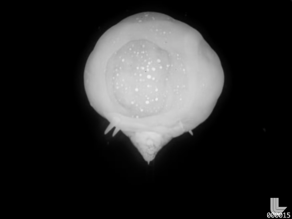
The photos Taylor saw were probably just like the photo above. Note that there is a time stamp and a distance scale. That’s important, because those quantities let one “measure” the time the blast has been developing (from, effectively, a point) and the size (or radius ) of the “spherical” shape. Yes, you have to treat the top part as part of a spherical shape and hope the interaction with the ground doesn’t affect that too much. But the thing with hope is you might as well see how far it takes you before you lose it.

That’s actually quite the complicated fluid dynamics problem. But dimensional analysis is powerful. Figuring the density of air might have something to do with the size (since the blast has to push out all of that surrounding air) one can fiddle around with just those three quantities (, , ) to obtain a combination that has dimensions of energy, .

Following Taylor, we can get out a ruler. I estimated the diameter at , which almost certainly contains more precision than I’m justified to retain. This is an example where things are so crude that significant experimental effort is not rewarded—the theorist’s dream! The expansion time is , and the STP density of air is . Put all that into , and you get . A number that big means we’re probably using silly units. We can take the old-school approach of looking up the conversion to kT of TNT (it’s ) or just ask Google directly. Either way, we’re probably using Google, and we get . The source on that photo estimates . Not bad for the minuscule effort!

I think I saw this ten years ago. Fast forward a few years, and I saw this again in Zee’s entertaining Fly by Night Physics. There, Zee goes through the same sort of argument, arriving at the same order-of-magnitude result. But he also makes the very sound point that one would get a better estimate by performing regression on a series of measurements. After all, think about how many introductory labs eventually coerce the student to performing linear regression on some data set before yielding the “final” answer. If one goes to the source for that image above, you can click “next” or “previous” to scroll through shots at different times. That’s handy.

The Trinity photos are pretty famous, and Taylor beat us all to the punchline. However, a few years ago, Lawrence Livermore National Labs posted a nice collection of recently declassified, high-resolution test footage from the 1950’s. Given that Wikipedia has an extensive list of US nuclear tests with estimated yields, one is well equipped to try out the method and see how it does in the wild.

Frame 15 from Tesla shot, Operation Teapot (source)

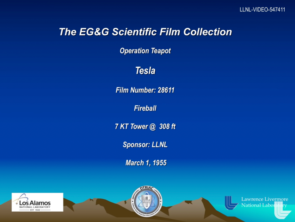
I spent a few minutes scrolling through the footage, and the Tesla shot from Operation Teapot (1955) was the first one I found that looked amenable to this kind of crude analysis. The good news is that the footage includes the frame number in the lower-right corner. The video comment also indicates the video was shot at “around 2,400 frames per second.” The ambiguity is ominous, but crude methods are robust to uncertainty. So we have a time stamp for each frame.

The less-than-good news is that there’s no length scale handed to us like in the Trinity photos. Fortunately, the title frame just happens to divulge that the device was detonated from atop a 308-ft-tall tower. That’s about 90 m, and it corresponds to the distance between the ground and the blast center.

Title frame for Tesla shot, Operation Teapot (source). From here we get the length scale and the (approximate) yield.

So in principle, we can just grab a frame and use the appropriate and to estimate the blast yield. But since there are so many usable frames here we can also take advantage of all the information, ultimately performing a fit to get a better estimate. This procedure has “tedious” written all over it, but there’s no reason one couldn’t do this “by hand” (like Taylor allegedly did) with each frame from the YouTube video. That’s one path. But I used LoggerPro because I happen have it installed. Any primitive video analysis software is going to save some time.

In LoggerPro, the green line sets the scale (90 m), the yellow crosshairs show the origin, and the blue dot represents the point being tracked (edge of blast).

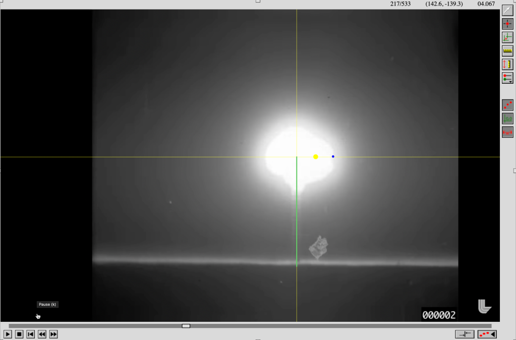
Back at HPU, we had a bunch of introductory labs involving video analysis in LoggerPro. It’s remarkably easy to use. After importing the video, one just sets the origin, scale, and frame rate before clicking on a point in each frame to track. It’s so easy, even I can do it and get decent results. The high-speed 1950’s film quality leads to a lot of judgment calls about where the edge is, but the idea behind using all the points is that random errors are going to cancel out (roughly, hopefully). Also, it turns out that taking a screen recording of the YouTube video playing is “good enough,” but you’ll probably get some duplicated frames because the recording won’t be perfectly in phase with the playback. Quick and dirty for the win.

Once all the points are collected, LoggerPro (or any tool you use) should have a collection of and values. If you’re using LoggerPro, you can do the rest there or just export and use Excel or Python (or whatever is hip these days). Since we expect , it means we should expect a linear relationship between and . So we plot versus and observe the strikingly linear relationship that emerges.

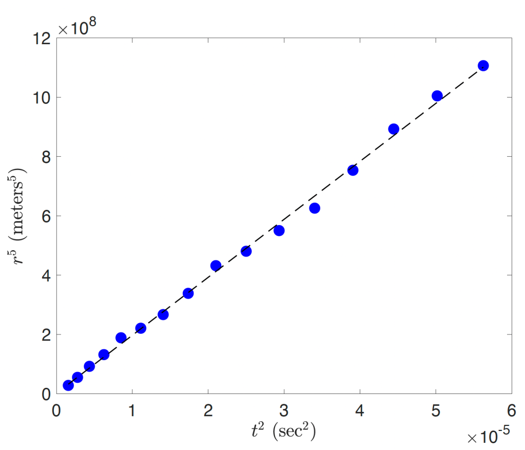
Use your favorite tool to perform linear regression, and that slope should correspond to where is some unknown (dimensionless) constant we must inherit as the cost of using dimensional analysis. We don’t know what is, but generally it’s “of order one,” . That doesn’t mean it’s necessarily close to one. It could be or or any number of exotic constants. But it’s probably not going to be or . We’re looking for a crude estimate: is the yield a few kilotons or a few hundred kilotons? So really, we’re just estimating . Behold, the street-fighting approach.

In this case, the slope works out to . Converting this to energy, and using gives , or . That’s compared to the quoted, so it’s quite good agreement. If anything, it suggests that we’re lucky and , at least for the conditions of these two tests.

To be fair, I tried the same thing with another shot and got compared to a quoted value of . I suppose it’s possible that the government underreported or miscalculated the yield, but certainly not to this extent. More likely, that dimensionless constant is some function of parameters that doesn’t vary much from unity for low yields. At higher energies, other physics might become more relevant, leading to a different (apparently smaller) value for . It’s possible one could comb through these videos and work out the effective for a range of yields to see whether or not there’s a simple functional form. Unfortunately, most of the bigger yields seem to be air drops or near-surface detonations. In either case, there’s no easy way to set a length scale in the video. But there are a number videos for other low-yield devices set off from towers, so it would still be interesting to see if holds up for some of those.