
Introduction
Hopefully, this will be the first of a series of posts about incorporating quantum computing into an undergraduate quantum mechanics course. It was during the first week of classes two years ago when I discovered the IBM Quantum Experience, which allows anyone to access actual quantum devices on the IBM cloud for free. At that point, I did not have the bandwidth to do much more than fiddle around with the hardware in my limited free time and encourage a few students to try it out as part of their course projects. Now that I’ve had some time to prepare to teach the course again, I’m ready to actually integrate this incredible resource into the class. For the uninitiated (as I was very recently!), Qiskit is an open-source software development kit (SDK) that allows users to access cloud-based, IBM quantum hardware. I feel like this needs to be said again: you can access IBM’s quantum computers using a free Python-based SDK.
Some caveats to what follows: I’m teaching a mix of juniors and seniors who have had experience using Glowscript since their first physics course and experience using Jupyter notebooks since at least their sophomore-level modern physics course. Computation is an integral part of our curriculum, so it’s not as daunting to jump into using Qiskit as it would be if this were their first exposure to Python. Also, our program is somewhat unusual in that we have a lab section associated with each of the four core upper-level courses (QM, E&M, Classical Mechanics, Thermal Physics) instead of having a dedicated “advanced lab” course. That’s two hours each week on top of the four contact hours for “lecture” that can be used for computation. Probably two thirds of that time was devoted to computational endeavors the last time I taught this course, and I expect a similar amount of time being used for that this semester. It would be a lot harder to incorporate quantum computing without those “extra” two hours per week.
To conclude this preamble, I should also note that IBM has a Quantum Educators program. One potential roadblock to using this technology in an in-person class setting is that you are competing with pretty much everyone else in the world for time on these devices–turns out that a lot of people are interested in quantum computing! As part of the Educators program, you get access to hardware not available to the general public as well as the ability to reserve priority access on several devices. I highly recommend that anyone looking to use this technology in a course apply for the Educators program. For in-person (time-constrained) activities or demonstrations, the Quantum Educators Program has been a life saver.
Motivation
So why incorporate quantum computing into an otherwise fine acceptable course on quantum mechanics? For starters, this is an incredible opportunity for students to get experience with cutting-edge technology. Most physics majors will not pursue academic careers in physics. If there were ever a way to make quantum mechanics relevant to future software engineers and data scientists, this is it.
From a more academic point of view, quantum computers provide an easily accessible experimental component to highly abstract topics like spin, entanglement, and quantum time evolution. It’s certainly possible to probe such physics experimentally, but this generally entails expensive equipment. For free, students can perform legitimate experiments on state-of-the-art quantum hardware.
I should also mention that I’m fairly new at all of this. Anything I write about is a work in progress. Fortunately, it’s quite fun to explore this technology. If you’d like to follow along within a Jupyter notebook, you can download a notebook here. For ease of reading (but with a total lack of functionality), an HTML depiction of the notebook is located here. That Jupyter notebook is a sample of what students are given. This will all be organized on GitHub at some point.
The textbook for this course is employs a spin-first approach, so we are talking about the Stern-Gerlach experiment on the first day and using the excellent SPINS program to simulate various experimental setups. For example, we might attempt to predict the measured counts for the following arrangement of spin analyzers if 

 is measured twice while
  is only analyzed between the two successive measurements. Students also show that the (expected) final counts change dramatically if only the “spin up” sample from the middle analyzer is fed into the final measurement.
 Now, I like this program a lot. It’s fairly easy to use, and it doesn’t require any programming. Even its quirks are charming. But when we get to entanglement and multi-particle states, students essentially have to write their own simulator in Python. The last time I taught this course, students built such a program in stages with the first step being to create a program that reproduced the kinds of results they found using SPINS. But that felt really contrived. Why reinvent the wheel in a clunkier way? Instead of dragging students through that tedious process again, we can just use IBM hardware to perform the experiment and analyze the actual data.
Students install Qiskit on their own laptops and set up their own IBMQ accounts, and this takes some a lot of time. In the end, most ended up just using the excellent IBM Quantum Lab to use Qiskit in IBM’s cloud-based Jupyter lab. So on the first day of using Qiskit, I just had students go through a tutorial that introduces the correspondence between “spins” and “qubits” and walks them through how one can “measure” the spin projection along a particular direction. It’s a bit of work for a pretty modest task. But this is a nice opportunity to spin (pun intended) the fairly abstract idea of quantum states from an experimental point of view.
The textbook assigns the ket 


Our first quantum circuits
To get students to go through the basic processes with absolute minimum complexity, we start out with the following incredibly basic circuit:

All this does is to initialize a qubit in
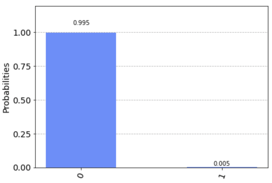
ibmq_belem v1.0.18, one of the IBM Quantum Falcon Processors): most of the qubits are measured to be in the state ‘0’ corresponding to the spin state , while ‘1’ corresponds to . A central idea in quantum mechanics is that the outcome of a particular measurement event is essentially unpredictable. The outcome is constrained to be one of the eigenvalues of the operator corresponding to this observable. The best we can do to predict outcomes is to work out a probability distribution. Experimentally, this only emerges after many measurements are made on identically prepared systems. Running a job actually consists of repeating a circuit many times with the default number of such “shots” set to 1024. Qiskit’s built-in histogram function turns the raw counts into a visual representation of the underlying probability distribution.
The other thing students can observe from this incredibly simple simulation is that present-day quantum computers are not error free. When they run this circuit on the simulator, the results show that the counts are entirely in the ‘0’ state. What else could happen? We just prepared a bunch of copies of the 
Introducing quantum computing in this course is motivated by the ability to simulate quantum mechanical systems. So what we do doesn’t really rely on the traditional background one builds up to study quantum computing (theory of computation, logic gates, and so on). Consequently, I’m introducing topics only as I need them, and so some of this might seem to arranged strangely. For example, the first gate we really use is a rotation gate. Why? Because we need it to measure spin projection about arbitrary axes.
What I really love about using these devices is that you have to think like an experimentalist. This does not come easy to me, but that also makes it interesting. One apparent roadblock to simulating a complex Stern-Gerlach setup is that we only have access to measurements in the “computational basis.” That is, we can only measure spin projection along the 


 , we can rotate the system so that a measurement of the rotated state in the computational basis is equivalent to a measurement of the actual state in the desired basis.
Students are shown that “rotation gates” exist which can perform exactly such a rotation by a specified angle about a specified axis. As a simple example, we can measure 


Students know from the SPINS program that measuring 
 on the state ( in quantum computing conventions) using QASM simulator and quantum hardware (
ibmq_quito v1.0.18, one of the IBM Quantum Falcon Processors)At this point, I introduce the general 


The general 

Now once students string together circuits to (a) generate this state and (b) measure one of the three spin operators, they have to turn the resulting counts into spin expectation values. At the end of the day, these simulations return a set of counts. I think it’s a valuable experience for students to work with these raw counts and compute experimental values for quantities which can be computed theoretically. Also knowing that we’re going to talk about the Heisenberg Uncertainty Principle in the coming days, it’s crucial that students also quantify statistical uncertainty for these results. The expectation value is a simple average. From the counts, students obtain 


A crude measure of statistical uncertainty in the estimate of this average is provided by the variance via 

I think this is an interesting point, because 


 )
) from
ibqm_casablanca v1.2.30, one of the IBM Quantum Falcon Processors.These can be compared to theoretical predictions 


Closing thoughts
By the end of this lab sessions, students are able to initialize arbitrary spin states 
References
- IBM Quantum Experience
- Qiskit Textbook
- J. Body and G. Guzman, “Calculating spin correlations with a quantum computer,” Am. J. Phys. 89(1), 35-40 (2021).
- D. McIntyre, C. Manogue, and J. Tate, Quantum Mechanics, Pearson, 2013.
- SPINS program
I acknowledge the use of IBM Quantum services for this work. The views expressed are those of the author, and do not reflect the official policy or position of IBM or the IBM Quantum team. Additionally, I acknowledge the access to advanced services provided by the IBM Quantum Educators Program.

3 thoughts on “IBM Quantum/Qiskit in QM Part I: Single Spins”