
You sit on a swing of length 

I’m gearing up to teach junior/senior-level classical mechanics again in the fall and remembered this half-baked idea from the last time I was teaching this course. My department is fortunate enough to have several TeachSpin torsional oscillators at our disposal, and I’ve used them for the lab component in this course. Most basically, these devices are experimental realizations of a simple harmonic oscillator with a really high Q-factor and a natural frequency on the order of seconds. Students can cook up experimental realizations of all the standard harmonic oscillator theory from this course with a really nice device they can touch and see working. It’s great for that.
But I’m repeatedly taken aback by all the non-standard stuff one can explore with this device. For starters, it’s actually easy to introduce three types of drag: sliding (constant) friction, viscous (proportional to velocity) drag, and high-Reynolds number (quadratic) drag. The linear drag is the only one students typically encounter in textbooks, presumably because it’s the only case with a clean, analytic solution. There’s a number of AJP/EJP articles about dealing with these special cases in great detail (see here, here, here, here, and references therein for starters). In the slow-dissipation limit, where only a small fraction of the energy is lost to friction during each cycle, it’s possible to obtain the trajectory approximately for arbitrary drag. We have a really nice lab where students investigate the validity of this approximation by comparing to a numerical solution, and then they end up doing the experiment to confirm that the approximate solution works pretty well in the experimentally-relevant range of parameter space.
Back in 2020, I saw David Van Baak give a talk at the AAPT Summer Meeting about using the torsion oscillator to investigate parametric resonance. In a nutshell, if the resonant frequency of an oscillator “wiggles” slightly at twice the resonant frequency, the oscillator’s amplitude increases. The TeachSpin oscillator can be tweaked to realize this phenomenon, and as I recall, the data looked pretty impressive. But how to model it? But how to model it without some fairly elaborate analysis involving the dreaded Mathieu functions?
Quick side note: here’s a great AJP article for learning about Mathieu functions.
At the top of this post is a homework question from when I was a TA for this course as a graduate student. The official textbook was Landau and Lifshitz with a generous dose of Arnold. I put more work into keeping on top of this class than I did in some of my own classes. But what a ride it was. As it turns out, I stayed up all night trying to resolve that question with exact analysis and got nowhere close to having physical insight. I suppose what follows represents some growth.
The classic example of parametric resonance is the aforementioned swing situation: how does one increase the amplitude while swinging on an ordinary playground swing? Intuitively, children (and some adults) know exactly what to do: “pump.”

The above cartoon depicts various poses one can take during a swing. But it’s not terribly descriptive, because one might vary the pose depending on the cycle. The question of interest here is whether physics suggests an optimal position for each point in the full (forward + backward) swing cycle. For that, we need a model.
Toy models make things as simple as possible, but not simpler. The leg motion suggests a double-pendulum-like system, but that’s fairly complicated to analyze. In essence, pumping legs has the effect of shifting the center of mass up and down along the radial direction aligned with the chains of the swing. So taking a cue from the problem stated at the top of this post, let’s just consider a simple (point mass) pendulum in which the length varies periodically at some arbitrary (angular) frequency 


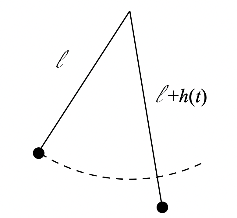
The “parametric resonance” arises from the natural frequency of this oscillator being 

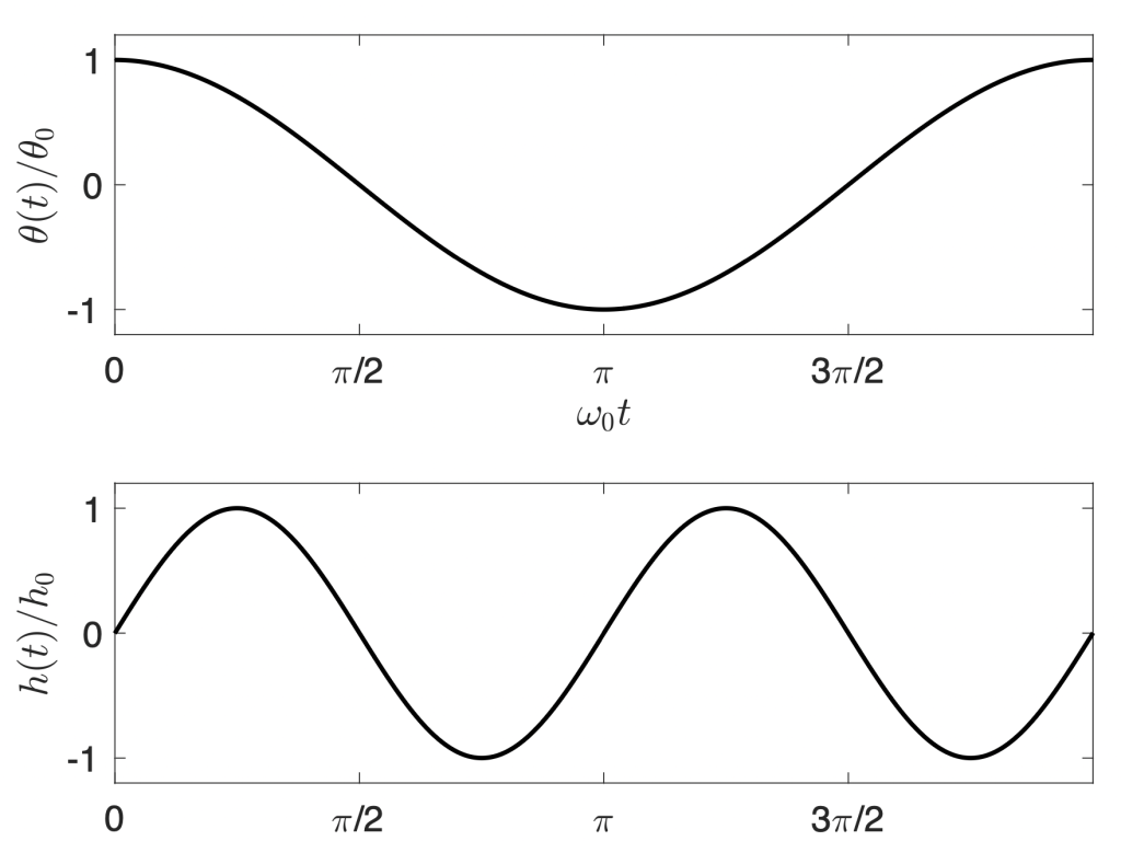
Even this simple model leads to a pretty complicated equation of motion. The beauty of physical models is that they allow one to make reasonable approximations to simplify the math. For example, an oscillator with a slowly increasing amplitude could reasonably be expected to have the angular behavior given by

Here it’s assumed that the variation of the length 


Packaging the solution as a time-dependent amplitude multiplied by a simple cosine function also works when one looks for the solution of a damped oscillator with arbitrary types of drag. For this more complex situation, we employ a Lagrangian to obtain the equation of motion:
![\displaystyle L = \frac{1}{2}m\left[\dot{x}^{2} + \dot{y}^{2}\right] - mgy = \frac{1}{2}m\left[\dot{r}^{2} + r^{2}\dot{\theta}^{2}\right] - mgr(1-\cos\theta).](https://s0.wp.com/latex.php?latex=%5Cdisplaystyle+L+%3D+%5Cfrac%7B1%7D%7B2%7Dm%5Cleft%5B%5Cdot%7Bx%7D%5E%7B2%7D+%2B+%5Cdot%7By%7D%5E%7B2%7D%5Cright%5D+-+mgy+%3D+%5Cfrac%7B1%7D%7B2%7Dm%5Cleft%5B%5Cdot%7Br%7D%5E%7B2%7D+%2B+r%5E%7B2%7D%5Cdot%7B%5Ctheta%7D%5E%7B2%7D%5Cright%5D+-+mgr%281-%5Ccos%5Ctheta%29.&bg=ffffff&fg=222222&s=0&c=20201002)
The Euler-Lagrange equation for the angular coordinate yield
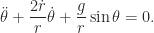
Under the small-angle approximation, 


To keep things PG, I’ll just point out the broad strokes of the calculation. Taking the energy of the pendulum, 

Using 


Equating the two expressions, and performing some simplification gives the equation of motion for the amplitude
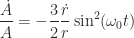
Given that 

Now we could deal with this mess, but we don’t actually have to solve the equation as written. In this case, at least, we can isolate the important part. To do so, let us proceed as if we wish to solve it by integrating both sides. Supposing the swing starts from some initial angular displacement 

If one unpacks the integrand and uses 

Now if 

Being proportional to 


![\displaystyle \theta(t) = \theta_{0}\exp\left[\frac{3\sqrt{g}h}{4\ell^{\frac{3}{2}}}t\right]\cos\left(\sqrt{\frac{g}{\ell}}t\right)](https://s0.wp.com/latex.php?latex=%5Cdisplaystyle+%5Ctheta%28t%29+%3D+%5Ctheta_%7B0%7D%5Cexp%5Cleft%5B%5Cfrac%7B3%5Csqrt%7Bg%7Dh%7D%7B4%5Cell%5E%7B%5Cfrac%7B3%7D%7B2%7D%7D%7Dt%5Cright%5D%5Ccos%5Cleft%28%5Csqrt%7B%5Cfrac%7Bg%7D%7B%5Cell%7D%7Dt%5Cright%29&bg=ffffff&fg=222222&s=0&c=20201002)
With such brutal approximations involved, it’s important to think about the validity of this simple result. The expression above assumes a tiny change in the center of mass of the swinger and also that the amplitude is also fairly small. It’s going to break down. Exponential growth of anything doesn’t last indefinitely, but it’s a useful model at short timescales.
To touch base with the problem posed at the top, we can set 

For what it’s worth, this works out to about 2.8 seconds for the parameters in the original question. That can be compared to the natural period of the swing itself also being 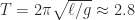
But the fun happens when we go beyond “the answer.” The approximations leading to this result escalated pretty quickly. Is there any reason to trust the conclusion? For starters, we can look at the expression itself. Dimensional analysis doesn’t let us guess the answer here since there’s a dimensionless constant 


It’s also straightforward to integrate the equation of motion numerically. In this case, one doesn’t have to make any approximations (


An impressive number of papers in the late 20th century have been devoted to analyzing the motion of a child on a swing with varying levels of sophistication. This one from 1998 has a pretty extensive list of references, but you can find a ton of them by just searching “swing motion” on the AJP site. Most of these works do more than to throw a cosine function into the pump function and see what happens. The article of Wirkus, Rand and Ruina linked above is probably my favorite, as it uses a step-function to model different strategies for pumping and links the functional forms to the types of sitting and standing approaches to actually pumping a swing. But the moment step functions enter a problem like this, the only viable course of action is a numerical approach.
So what’s the point in the silly cosine function we used here? It doesn’t closely resemble the actual motion of a real-life child who increases the swing amplitude almost effortlessly. It helps to go sit on a swing and observe how we naturally do this, but there’s also a great Sixty Symbols video on this. The cosine makes sense from the pragmatic point of view of trying to get as far as possible analytically while still preserving some essence of the original system. That’s the idea of a toy model. Introducing some type of periodic drive—which is the core of a pump, common to all approaches—the resonance that occurs when the pump frequency is twice that of the empty swing just pops out. Driving the system on resonance, the characteristic exponential growth is also seen. The quantitative predictions here likely don’t hold up to close scrutiny when compared to an actual child swings. But the underlying mechanism for how something like this happens is easily seen.
It’s a fun exercise to think about how 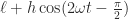

I love this! I think I’ll be firing up Mathematica tonight to have some fun with this approach.
LikeLike
Thanks for reading! Curious to hear what happens when you break out the big guns.
LikeLike